Loading...

Vektor 1
Quiz by Fyna
Customize this quiz to suit your class
Instantly translate to 100+ languages
Tag the questions with any skills you have. Your dashboard will track each student's mastery of each skill.
Give this quiz to my class
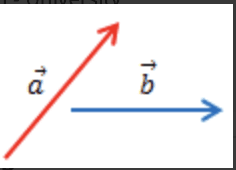
Diketahui dua vektor seperti pada gambar berikut...
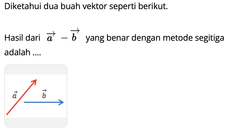


Diketahui dua vektor seperti pada gambar berikut...


Pernyataan yang benar dari gambar vektor di bawah adalah...
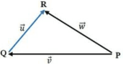
Secara geometri, dua vektor atau lebih dapat dijumlahkan dengan metode berikut ini...
Diketahui vektor sebagai berikut